System dynamics example
As an example of systems dynamics simulation, we can take the famous Bass diffusion model which is mostly used in forecasting the new products' sales.
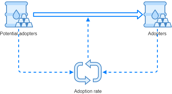
To understand the diffusion of a product, we can think about potential buyers on the one hand and persons who are already using the product on the other hand. At the beginning there will be no users of our product. We start with marketing activities, and as time passes, more and more people will buy the product. For a start, we can observe the number of adopters, that is people who already purchased the product, and people who will, supposedly, buy a product at some latter time.
Potential adopters are "transiting" to adopters at some adoption rate, which is the number of new adopters in a given time period, usually a year. The adoption rate is changing in time, it is not constant. According to the idea of Bass model, this adoption rate is a result of two factors - imitation and innovativeness. People are usually imitating other users, however there are others who are innovative, interested in that kind of products and adopt a novelty when they learn about it, for instance by marketing activities.
Model description
Bass model thus incorporates two parameters, coefficient of innovation p and coefficient of imitation q. We can observe the changing adoption rate by following the queation
rate = p·P + q·P·A/(P + A)
where P is the number of potential adopters and A is the number of adopters. As mentioned above, we expect that the number of potential adopters will slowly drop because people will become adopters.
As an example, we can use the following paramters, with 1000 potential adopters at the beginning:
p = 0.0560
q = 0.5666
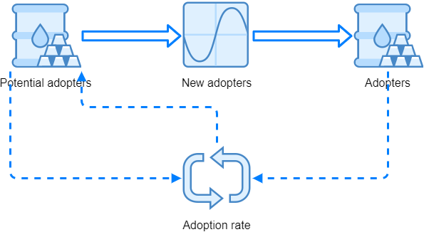
Following the above we can start to build the model with Spry. We need two stock elements to hold the system state, that is the number of potential adopters P and adopters A in a particular moment. Because the adoption rate depends from these states, and states depend from the rate, we have a feedback loop. This can be seen from a diagram that we can draw like this:
Model development
We start with the clock which defines 15 years of simulation time like this:
| A | B | C | |
|---|---|---|---|
| 1 | Clock: | =syClock(,15) | |
| 2 |
Then we prepare the potential adopters and adopters stocks in cells B2 and B3, respectively. For starters, we can just scaffold the model by entering zeroes for their arguments InflowRate, OutflowRate, DiscreteInflow and DiscreteOutflow.
For potential adopters in B2 we can already set the InitialValue to 1000 - this represents the number of potential adopters at the beginning of simulation time:
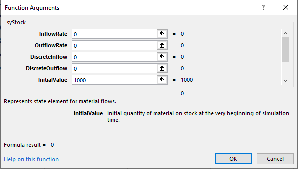
InitialValue argument should be 0 for adopters since there are none at the beginning, so we have:
| A | B | C | |
|---|---|---|---|
| 1 | Clock: | =syClock(,15) | |
| 2 | Potential adopters: | =syStock(0,0,0,0,1000,B1) | |
| 3 | Adopters: | =syStock(0,0,0,0,0,B1) | |
| 4 |
Of course, syStock() functions should refer to the simulation clock with their TimeNow argument as all other simulation elements do. After that, we can add p and q paramters (innovation and imitation coefficients) and enter the formula for adoption rate as:
| A | B | C | |
|---|---|---|---|
| 1 | Clock: | =syClock(,15) | |
| 2 | Potential adopters: | =syStock(0,0,0,0,1000,B1) | |
| 3 | Adopters: | =syStock(0,0,0,0,0,B1) | |
| 4 | p | 0.0560 | |
| 5 | q | 0.5666 | |
| 6 | Rate: | =B4*B2+B5*B2*B3/1000 | |
| 7 |
The feedback loop
Because the adoption rate is a rate, it can be directly used in syStock() elements as InflowRate or OutflowRate. The number of potential adopters will get lower and lower in simulation time, so we use the adoption rate as OutflowRate in this case. The adopters group will get bigger and bigger, so we can use adoption rate as adopter's syStock() argument InflowRate. This could be done by changing the formulas in B2 and B3, directly referring to the rate in B6:
Potential adopters (B2): =syStock(0,B6,0,0,1000,B1)
Adopters (B3): =syStock(B6,0,0,0,0,B1)
However, if we do that, we have a problem of circular references. Our rate formula is referencing cells B2 and B3, so we have to implement the feedback loop in some other way and not by direct cell references - syLoop() element can come to the resque. syLoop() takes two arguments: the first argument is the feedback loop name, and the second argument is the value to be send to state elements. In our case, we can put this formula in cell B7:
Loop (B7): =syLoop("Rate",B6)
After that, we can directly refer to the name of the feedback loop in our syStock() elements, so we get:
| A | B | C | |
|---|---|---|---|
| 1 | Clock: | =syClock(,15) | |
| 2 | Potential adopters: | =syStock(0,"Rate",0,0,1000,B1) | |
| 3 | Adopters: | =syStock("Rate",0,0,0,0,B1) | |
| 4 | p | 0.0560 | |
| 5 | q | 0.5666 | |
| 6 | Rate: | =B4*B2+B5*B2*B3/1000 | |
| 7 | Loop: | =syLoop("Rate",B6) | |
| 8 |
As we can see in our example, syStock() and syState() elements can directly use the loop names by their InflowRate, OutflowRate, DiscreteInflow and DiscreteOutflow arguments.
Outcomes
To check if our model works, we use syOutcome() element. Choose a free cell with enough space below it - we need a range of cells that is at least 16 rows high for the results - and set the syOutcome() parameters like this:
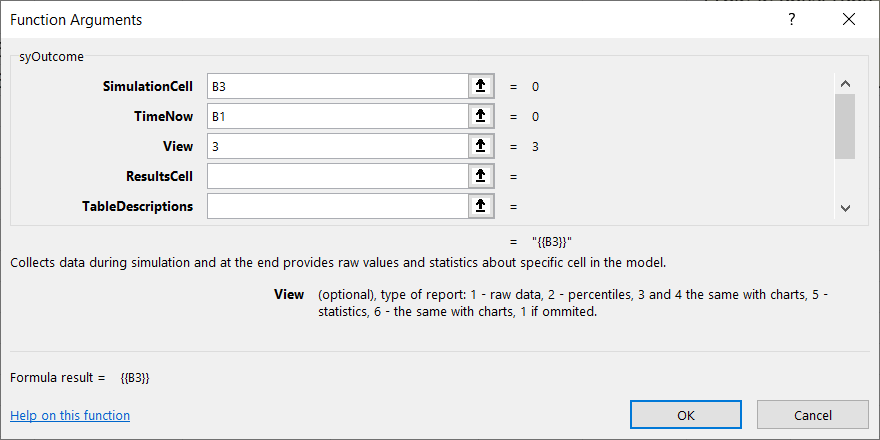
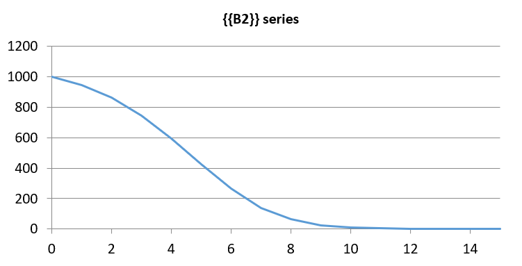
This outcome element will display the number of adopters in time after we run the model. Argument View = 3 displays the results (number of adopters in each time step) and also displays a chart like this:
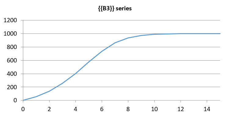
Of course we should also check the potential adopters in a similar way - the diagram should look like:
Outflows
In adopter's stock we used adoption rate as InflowRate argument. Because we are dealing with system dynamics simulation, it is more appropriate to somehow create a "pipeline" so that the actual OutflowRate from potential adopters' stock is respected directly by adopters' stock element.
syStock() function by default displays the current state (value, level) of the stock. However, if we are interested in stock's outflow rate or outflow quantity (the quantity that went out from the stock in the last time interval) we can use syStockOutput() function that points to our syStock(). With this in mind, we can introduce these changes:
| A | B | C | |
|---|---|---|---|
| 1 | Clock: | =syClock(,15) | |
| 2 | Potential adopters: | =syStock(0,"Rate",0,0,1000,B1) | |
| 3 | New adopters: | =syStockOutput(B2,3) | |
| 4 | Adopters: | =syStock(B3,0,0,0,0,B1) | |
| 5 | p | 0.0560 | |
| 6 | q | 0.5666 | |
| 7 | Rate: | =B5*B2+B6*B2*B4/1000 | |
| 8 | Loop: | =syLoop("Rate",B7) | |
| 9 |
Above, we inserted a row between adopters and potential adopters stocks and used the formula:
New adopters (B3): =syStockOutput(B2,3)
The formula is referring to potential adopters syStock() in cell B2. The second parameter sets the desired output of syStockOutput() to be the outflow rate of observed syStock(). This outflow rate can be directly used by adopters' syStock() as InflowRate:
Adopters (B4): =syStock(B3,0,0,0,0,B1)
There's also another option - we could use the outflow quantity in the last timestep by using these formulas:
New adopters (B3): =syStockOutput(B2,1)
Adopters (B4): =syStock(0,0,B3,0,0,B1)
Tips
Above, we set the syStock() third argument DiscreteInflow to "inject" into it the quantity that came from potential adopters by syStockOutput(). This can be conceptually described as:
You can download this example from GitHub.