Model with optimization
Inventory models typically deal with the challenge of optimal ordering, both with the quantity of items ordered and the timing of orders. When searching for the solution, one of the possibilities is to use discrete-event simulation, however we'll use the stock element to represent the inventory (the number of mixers in our store) and discrete events to change the state. Although our example is very simple, it can be enriched with additional complications.
The challenge
Our task is as follows: we have a building material store that sells concrete mixers. According to our experiences, we can sell up to 4 mixers per day, but it can happen that we sell none. Every couple of days we check our storage to see how many mixers are missing to fill up our inventory. Because of their size we only have space for up to 11 mixers, so we make an order for the difference. It takes one to three days for the suuplier to deliver the mixers.
Because of the delivery costs we'd like to reduce the number of orders, however we could run out of stock and loose the income. Our task is to estimate the optimal number of days between orders (we will limit the search from 1 up to 10 days between orders). We also assume that the cost of each order is 1, and the cost of each item not on stock is 0.5. We decide that we'll simulate one business month of our store and check these costs. We start with 11 mixers on stock.
Setting up the data
According to our historic data, we arranged the demand probabilities in spreadsheet column M and delivery delay probabilities in column N, whereas column L represents corresponding number of items for demand and the number of days for delivery delay:
| L | M | N | ||
|---|---|---|---|---|
| 1 | Items / Days | Probabilities (demand) | Probabilities (delivery) | |
| 2 | 0 | 0.10 | ||
| 3 | 1 | 0.25 | 0.60 | |
| 4 | 2 | 0.35 | 0.30 | |
| 5 | 3 | 0.21 | 0.10 | |
| 6 | 4 | 0.09 | ||
| 7 |
These historic data can be used in our simulation to generate every day demand, and also the delivery days. We'll use syRandomDiscrete() function to arrange for the random number generator which respects discrete probability distribution. For ur data, we'll set the parameters as follows:
B2: =syRandomDiscrete(L2:L6,M2:M6) for demand and
B3: =syRandomDiscrete(L3:L5,N3:N5) for delivery delay
Business month lasts 25 days, so we arrange the following formulas:
| A | B | C | |
|---|---|---|---|
| 1 | Clock: | =syClock(,25) | |
| 2 | Daily demand: | =syRandomDiscrete(L2:L6,M2:M6) | |
| 3 | Lead time: | =syRandomDiscrete(L3:L5,N3:N5) | |
| 4 |
The model
How to proceed? We can start with the inventory quantity, which is a state. Because we are clearly dealing with material, we can use the syStock() element. Sold mixers during each day can be easily removed from stock as a quantity of discrete removals, so we can just tie the Daily demand random number generator with stock's DiscreteOutflow - this will remove the demanded quantity of mixers from the stock, for each consequent day.
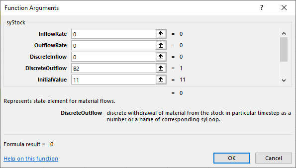
Besides the above arguments, we set the arguments LowestLevel to 0 and HighestLevel to 11, so that we get the following:
| A | B | C | |
|---|---|---|---|
| 1 | Clock: | =syClock(,25) | |
| 2 | Daily demand: | =syRandomDiscrete(L2:L6,M2:M6) | |
| 3 | Lead time: | =syRandomDiscrete(L3:L5,N3:N5) | |
| 4 | Inventory: | =syStock(0,0,0,B2,11,B1,0,11) | |
| 5 |
The incoming mixers, that is the mixers that are delivered to us, are a bit more complicated. Firstly, we have to establish the ordering schedule, then we have to calculate the quantity of mixers to be ordered when the time comes, and the mixers take 1 to 3 days to come to our store. The process can be depicted as follows:
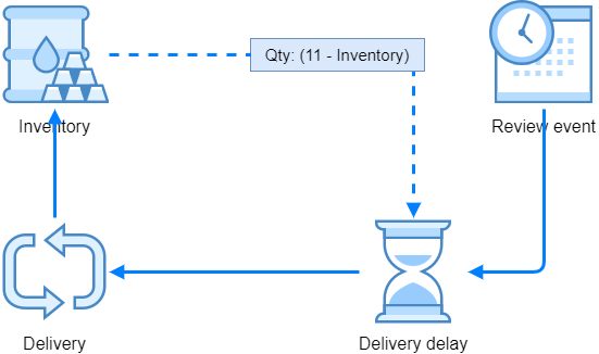
Because the system includes the feedback loop, we have to resort to syLoop() element to "deliver" our mixers to inventory. Namely, the quantity that should be ordered depends from the stock, and the stock depends from the ordered quantity.
Let's continue building the spreadsheet with the ordering schedule: we'll start with 5 days between orders, and the first order will happen by the end of the fifth day:
B5: =syScheduler(1/5,1,B1)
Then, we calculate the quantity to be ordered very easily:
B6: =11-B4
Since each syScheduler() event is expressed as 1, we can "schedule" the above quantity just by multiplying the syScheduler() result and the quantity as B5*B6. This result should be delayed by the number of days that we get from the random number generator in B3, so we have
B7: =syMaterialDelay(B6*B5,B3,B1)
The assumed unit of time in syClock() is a day, so both the syScheduler() and syMaterialDelay() are consistent with that. They both measure time in days - scheduler fires one event per 5 days (Rate = 1/5) and the delay uses days from random number generator (DelayTime=B3).
The only part that is now missing is the syLoop():
B8: =syLoop("Delivery",B7)
Then we close the loop with updating the stock:
B4: =syStock(0,0,"Delivery",B2,11,B1,0,11)
The core mechanism for our inventory model is done:
| A | B | C | |
|---|---|---|---|
| 1 | Clock: | =syClock(,25) | |
| 2 | Daily demand: | =syRandomDiscrete(L2:L6,M2:M6) | |
| 3 | Lead time: | =syRandomDiscrete(L3:L5,N3:N5) | |
| 4 | Inventory: | =syStock(0,0,"Delivery",B2,11,B1,0,11) | |
| 5 | Review event: | =syScheduler(1/5,1,B1) | |
| 6 | Order qty: | =11-B4 | |
| 7 | Delivery delay: | =syMaterialDelay(B6*B5,B3,B1) | |
| 8 | Delivery: | =syLoop("Delivery",B7) | |
| 9 |
We can check the functionings by using the syOutcome() elements, for instance:
| A | B | C | D | E | F | G | |
|---|---|---|---|---|---|---|---|
| 13 | {{B1}} | {{B4}} | {{B2}} | {{B5}} | {{B3}} | {{B7}} | |
| 14 | 0 | 11 | 1 | 0 | 1 | 0 | |
| 15 | 1 | 9 | 2 | 0 | 2 | 0 | |
| 16 | 2 | 7 | 2 | 0 | 1 | 0 | |
| 17 | 3 | 5 | 2 | 0 | 1 | 0 | |
| 18 | 4 | 2 | 3 | 0 | 1 | 0 | |
| 19 | 5 | 0 | 3 | 1 | 1 | 0 | |
| 20 | 6 | 0 | 1 | 0 | 1 | 11 | |
| 21 | 7 | 8 | 3 | 0 | 1 | 0 | |
| 22 | 8 | 8 | 0 | 0 | 1 | 0 | |
| 23 | 9 | 6 | 2 | 0 | 1 | 0 | |
| 24 | 10 | 4 | 2 | 1 | 2 | 0 | |
| 25 | 11 | 3 | 1 | 0 | 1 | 0 | |
| 26 | 12 | 0 | 4 | 0 | 1 | 7 | |
| 27 | 13 | 4 | 3 | 0 | 2 | 0 |
Column A is the clock and it shows the days - technically, the row 15 where the clock is 1 shows the state at the end of the first day and events that happened during the first day. Column B shows the inventory state, which is dropping by the daily demand in column C. During the first day, there was the demand for 2 mixers, so at the end of the day we have 9 remaining mixers.
Column D shows the order events which happen every 5 days. On the 5th day, the inventory was 0, that's why the ordered quantity was 11 mixers. Column F shows delayed quantity of items received, and we can see that the items ordered during the 5th day arrived in sixth day, because the delivery delay was 1 on 5th day when we made an order.
Likewise, next order happened on day 10, the missing quantity was 11 - 4 = 7, the delay time was 2 and we had 7 mixers available in day 12.
The inventory gets higher as soon as the items arrive, however because of the delay and the fact that on the same day new items are being sold, the quantity cannot reach the maximum of 11.
Decision variables
For our optimizaton task we need to establish the number of days in a month that we have zero inventory. This can be nicely done with syState() element which will count these days where we'll check if Inventory = 0. If this is true, we add the daily demand from cell B2 to our state. So we set:
B9: =syState(0,IF(B4=0,B2,0),0,B1)
Another part of the costs that we have with the inventory are the costs of each order, so we have to know how many orders are issued. We'll use another state:
B10: =syState(0,B5,0;B1)
This element counts the number of order events in a month. Lost profit per unsold mixer is 0.5 and the price of an order is 1, so we can prepare the decision formula as:
B11: =B9*0.5+B10
This will represent our cost function, the objective cell that we will try to minimize.
Because one realization is not enough (we have two random variables in the model, daily demand and delivery delay), we set the clock to 10 realizatios like:
B1: =syClock(10,25)
The formula in optimization cell B11 will provide different results during simulation time, and between realizations. For optmization purposes, we need an average of the final values across all realizations. Final value means the value at clock=25. One way to get the average of all realizations' final values is to use syOutcome() with the following settings:
=syOutcome(B11,B1,5,,1)
So, we are collecting the statistics for cell B11 (our objective cell), with View=5 we want descriptive statistics, and TableDescriptions=1 we'll get the names of descriptives, like this:
| G | H | I | ||
|---|---|---|---|---|
| 1 | {{B11}} | |||
| 2 | Average: | 11.9 | ||
| 3 | St. dev.: | 1.449137675 | ||
| 4 | Median: | 12 | ||
| 5 | Mode: | 12 | ||
| 6 | Minimum: | 9 | ||
| 7 | Maximum: | 14 | ||
| 8 | Kurtosis: | 1.1510636 | ||
| 9 | Skewness: | -0.334079358 | ||
| 10 |
This way of displaying descriptive statistics is meant for end users, however if we want to use one of the statistics for our optimization purposes, it's better to use syStatistic() instead of syOutcome(). So, if we want to have an average of the final values of optimization cell B11 across all realizations, we can use this setting:
=syStatistic(B11,B1,1)
The third argument Statistic=1 tells the function to return average value across all realizations. Before running the simulation, the syStatistic() function returns #N/A because the data is not available yet.
Another decision variable is the number of days between orders. Our goal is to find an optimal number of days between orders, so that the costs of orders and costs of zero inventory days are minimal.
For that purpose, we change the argument Rate of Review event's syScheduler() from 1/5 to 1/C5 like so:
B5: =syScheduler(1/C5,1,B1)
In this way, the cell C5 represents the number of days between orders, and can be used as variable cell during optimization.
Equipped by decision variables, our model looks like this:
| A | B | C | |
|---|---|---|---|
| 1 | Clock: | =syClock(10,25) | |
| 2 | Daily demand: | =syRandomDiscrete(L2:L6,M2:M6) | |
| 3 | Lead time: | =syRandomDiscrete(L3:L5,N3:N5) | |
| 4 | Inventory: | =syStock(0,0,"Delivery",B2,11,B1,0,11) | |
| 5 | Review event: | =syScheduler(1/C5,1,B1) | 5 |
| 6 | Order qty: | =11-B4 | |
| 7 | Delivery delay: | =syMaterialDelay(B6*B5,B3,B1) | |
| 8 | Delivery: | =syLoop("Delivery",B7) | |
| 9 | Days 0: | =syState(0,IF(B4=0,B2,0),0,B1) | |
| 10 | Order costs: | =syState(0,B5,0;B1) | |
| 11 | Total costs: | =B9*0.5+B10 | =syStatistic(B11,B1,1) |
| 12 |
Optimization
To do the optimization, Spry can be used in combination with Solver add-in. The idea of Solver is that it iteratively changes variable cells (such as our cell C5 with days between orders) according to constraints, observes the objective cell (in our case this is cell C11 with inventory costs) and searches for the optimal combination of variable cells values.
Every time Solver changes the objective cell, Spry has to run the complete simulation (all realizations). Because Solver cannot click on the Run button, we have to do this differently. This "buttin pressing" is the task of a special function called syExposeVariableCells() which takes a cell or a range of cells that Solver should change repeatedly, and Spry runs the simulation after each change.
We expose the variable cell in C5 like this:
D5: =syExposeVariableCells(C5)
The function returns the address of the exposed cell (or cells) in double-squared brackets, for instance [[C5]] After that, we can test the exposed cell just by changing the value in C5 (for instance, from 5 to 10) and entire simulation should run. We wait until it completes, and proceed with Solver settings:
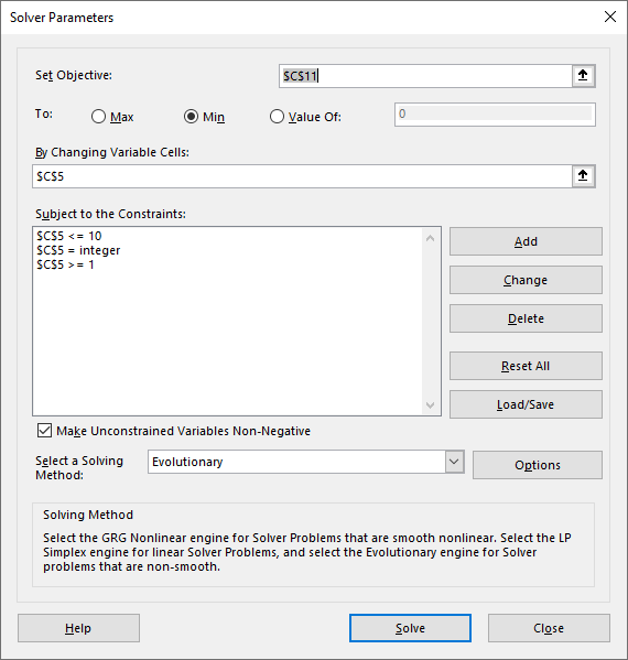
Objective cell is C11 with the costs where we search for the minimum value, variable cell is C5. We also set the constraints: we'll limit the number of days between orders to be positive and not more than 10. It should also be an integer value.
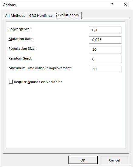
For models with stochastic variables (Monte Carlo simulation) where we expect non-linearity and local extremes it is suitable to use Evolutionary optimization method. We can use these specific options with this method in our case:
Tips
In this example we followed similar steps as before: we developed the core model, tested its inner mechanism if it works as expected, and continue with economic part of the model (estimation of costs). Finally, we used the model in combination with Solver.
You can download this example from GitHub.