A simple discrete-event model
We'll make first steps in Spry with a simple barbershop model. Customers are coming to our shop, roughly one customer per five minutes, and we need around 5 minutes per customer to perform full service. Under these assumptions we'd like to check whether we can serve all the customers without causing long queues in front of our shop. Discrete-event simulation is the best approach to solve our little problem.
In theory our case seems fine, because the frequency of arrivals corresponds to our service time, however we are a bit worried because of sporadic nature of arrivals and also of the service time. Could this sporadic nature be problematic, so that the customers will have to wait for the service and the queue will be longer and longer throughout the workday?
The clock
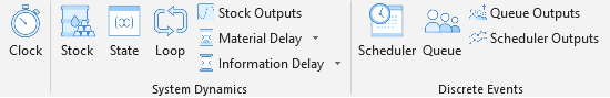
Dynamic models always have a clock, so let's start bulding our model with it. The clock is one of the simulation elements in Spry, and these are implemented as spreadsheet functions. Model's clock can thus be created with syClock() function. To make life easier, after Spry is installed there should be a new ribbon in Excel called Spry Simulation that lists all of the simulation elements:
To make our barbershop model easy to understand, we put a label "Clock:" in cell A1 and create a clock in cell B2 by selecting this cell and clicking on Clock button on the ribbon. The function wizard opens, inviting us to set the clock's parameters:
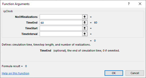
We'll start with simulation time of 60 minutes, that means we'll simulate the first 60 minutes of our barbershop, so we set syClock's argument TimeEnd to 60. Other arguments are optional, so we can just click OK.
This should be the result so far:
| A | B | C | |
|---|---|---|---|
| 1 | Clock: | =syClock(,60) | |
| 2 |
You'll notice that cell B1 displays 0 as a result in your spreadsheet. When firstly entered, Spry spreadsheet functions that represent simulation elements usually display zeroes. While we are designing the model, functions' return values are not important, they become important once we run the simulation. We only have to pay attention if the function returns error value (e.g. #VALUE!) when we enter it during the model design. This usually means that the arguments that we entered are not set according to the function's expectations.
Note
In design time, Spry functions usually return zeroes or other default values, they don't return any simulation results just yet. However, if a function returns #VALUE! or some other error, then you should check whether its arguments are entered as expected by function.
Model execution
Although pretty empty, our simulation model is technically ready to be executed! Click on the Run button in Experiment group and Spry will recalculate the model several times - the syClock will sequentially return values from 0 to 60 - from zero simulation time to the end of 60th minute. The recalculation will be done 61 times, for each timestep.
This clock ticking is too fast for us to observe. The purpose of syClock is that it provides the current simulation time to other simulation elements, and not for us to watch it. However, we can still monitor the processes in our model, including the clock, with syOutcome element. This element produces a table of all the values that some other element is generating during simulation time. This is true also for the clock itself.
To demonstrate this functionality, select cell A7, where the clock's values will be printed, click on Outcome button in Experiment group, and enter B1 as SimulationCell argument. This is the cell that syOutcome will gather the statistics for.
Note
Besides this, you can see that syOutcome's TimeNow argument is automatically set to the cell with the clock. Namely, TimeNow argument will tell syOucome that the simulation time has changed, in each timestep, and that it has to do the data gathering.
Now run the simulation and when it finishes, syOutcome will display a column of all the values that syClock returns from 0 to 60 minute.
| A | B | C | |
|---|---|---|---|
| 1 | Clock: | 60 | |
| 2 | |||
| 3 | |||
| 4 | |||
| 5 | |||
| 6 | |||
| 7 | {{B1}} | ||
| 8 | 0 | ||
| 9 | 1 | ||
| 10 | 2 | ||
| 11 | 3 | ||
| 12 | 4 | ||
| 13 | 5 | ||
| 14 | 6 | ||
| 15 | 7 | ||
| ⋮ | ⋮ | ||
| 67 | 59 | ||
| 68 | 60 | ||
| 69 |
As you can see, syOutcome by default prepares a table of the cell's results in each timestep. Simulation time starts at zero time and lasts until the end of the 60th minute. Spry pauses at each timestep (each simulated minute in our model), recalculates the model, while syOutcome elements note the state of cells that they are observing, and prepare the necessary tables at the end of simulation run.
The return value of syOutcome element in its cell is the name of the simulation cell that it observes, enclosed in mustaches {{}}. We are observing the clock in B1, that's why it outputs the cell address like {{B1}}.
Tip
syOutcome can be more descriptive than that - if you name the cell B1 as Clock, then the syOutcome would display {{Clock}}.
Before the simulation run, Spry checks if there are any data that can get overwritten by syOucome elements, and displays a warning if necessary. After you check the results, you can clear the output with button Clear on the ribbon.
The ribbon
The Edit button in Experiment group is used to edit the existing element in a selected cell - for instance, if you want to change the arguments of syOutcome() in A7, you select the cell and either click on Edit or Outcome button to display the function wizard. Of course, you can also edit the formula as usual without the wizard, Excel should display the formula and context help like this:
| 7 | =syOutcome(B1,B1) | ||

The Run button executes the simulation model. All the formulas in the model are recalculated once per each timestep. The model is the entire worksheet. While simulation is running, other worksheets and workbooks which may be open in Excel are not recalculated. Please also pay attention to the fact that a model can have only one valid syClock which is respected during the simulation run. If you put two or more clocks in the model, only the last one entered or edited will be respected by Spry. This is regarded as bad practice.
Note
Spry simulation model can have only one valid syClock which is respected during the simulation run.
The Clear button clears the results created by syOucome elements as displayed during the last run. If you repeatedly run the simulation, Spry will ask you if you are sure to overwrite the results if you keep them as they are. If you need them for later analysis, you can copy the whole range to some other location on the same worksheet or somewhere else in the workbook or other workbooks. syOutcome element can also put the results to some other location with ResultsCell argument.
Adding elements
Let's continue with our barbershop. Arrivals of customers can be regarded as events. Spry has an element that can generate events - syScheduler. Events occurring regularly (not sporadically) can be generated by setting syScheduler's argument Kind to 1 (regular events) or 2 (regular events, first of them happening at the beginning of period). syScheduler can also generate sporadic events (Kind = 3), so it's suitable for our purposes, but we can start with regular events, just to see how everything works, and after that we can proceed with stochastic complications.
syScheduler argument Rate defines the frequency, that is the number of events per unit of time. What is time unit in our model?
Unit of time is defined implicitly by syClock. When we set TimeEnd to 60, we defined 60 minutes for the clock to go from simulation start to simulation end time. The unit could also be seconds, days, years, etc. The chosen time unit (minute in our barbershop example) is important for the interpretation of the results, and for arguments that refer to time, like rates of change, arrival rates and similar. In Spry documentation we usually refer to this time unit as "assumed time unit".
According to our case, we add the syScheduler element by selecting cell B3, clicking on Scheduler button in Discrete Events group and entering the argument values, 1/5 as Rate and 2 as Kind. TimeNow is already set to B1, the cell with the clock. The value of Rate argument should be read as "one customer per five minutes":
| A | B | C | D | |
|---|---|---|---|---|
| 1 | Clock: | 60 | ||
| 2 | ||||
| 3 | Arrivals: | =syScheduler(1/5,2,B1) | ||
| 4 | ||||
| 5 | ||||
| 6 | ||||
| 7 | {{B1}} | {{B3}} | ||
| 8 | 0 | 0 | ||
| 9 | 1 | 1 | ||
| 10 | 2 | 0 | ||
| 11 | 3 | 0 | ||
| 12 | 4 | 0 | ||
| 13 | 5 | 0 | ||
| 14 | 6 | 1 | ||
| 15 | 7 | 0 | ||
| 16 | 8 | 0 | ||
| 17 | 9 | 0 | ||
| 18 | 10 | 0 | ||
| 19 | 11 | 1 | ||
By putting syOutcome(B3,B1) in cell B7 we can observe the events that syScheduler generated. Actually, syScheduler result value represents the number of events that happened in previous time interval. So, 1 at timestep 1 is read as "one event happening in the time interval from just after zero time until (and including) time 1".
Now, we have to somehow route the arriving customers to the barber. The barbershop can be represented by syQueue element. This element internally consists of one queue and one or more servers. The barber can be formally understood as a server that needs some time to provide the service for each customer.
syQueue expects two crucial arguments - the first one is InputValue which is interpreted as the number of events in the last time interval that are entering the element, and DelayTime which is the time in assumed time units that takes the server to process each customer - 5 minutes in our case. So, we can directly "feed" the syScheduler's output into the syQueue's InputValue argument like this:
| A | B | C | D | |
|---|---|---|---|---|
| 1 | Clock: | 60 | ||
| 2 | ||||
| 3 | Arrivals: | =syScheduler(1/5,2,B1) | ||
| 4 | Barber: | =syQueue(B3,5,B1) | ||
| 5 | ||||
| 6 | ||||
| 7 | {{B1}} | {{B3}} | {{B4}} | |
| 8 | 0 | 0 | 0 | |
| 9 | 1 | 1 | 0 | |
| 10 | 2 | 0 | 0 | |
| 11 | 3 | 0 | 0 | |
| 12 | 4 | 0 | 0 | |
| 13 | 5 | 0 | 0 | |
| 14 | 6 | 1 | 1 | |
| 15 | 7 | 0 | 0 | |
| 16 | 8 | 0 | 0 | |
| 17 | 9 | 0 | 0 | |
| 18 | 10 | 0 | 0 | |
| 19 | 11 | 1 | 1 | |
syOutcome in cell C7 shows the syQueue results, that is the customers that exited the barbershop during a particular time interval. As we see, customers are arriving regulary, and as the previous customer that has been served just leaves the shop, a new customer enters the barbershop doors.
Now we can add irregularities. syScheduler is capable of generating events randomly according to Poisson distribution. This can easily be done by setting its Kind argument to 3. The events are generated randomly while the rate of occurrence is respected and the actual average rate equals to the Rate setting. syScheduler thus becomes syScheduler(1/5,3,B1).
Besides this, we have to set the dispersion of the service time within syQueue by setting the Dispersion parameter to 1. In this case the DelayTime is regarded as a rate automatically (5 means one per 5 minutes on average). Dispersion argument is k parameter in Erlang distribution. According to this, we change syQueue to syQueue(B3,5,B1,1,,1).
Besides adding the last argument Dispersion, we also set the NumberOfServers to 1, because we only have one barber in the shop. If we don't set this argument, the default is infinite number of servers, so all our customers would be served without any waiting.
We already mentioned that the result from syQueue is the number of customers that left the barbershop in the last time interval. Before running the simulation, we can arrange one additional output from syQueue, because we are interested in the number of people waiting for the service. This can be achieved by syQueueOutput element which needs a reference to syQueue and the ID of data that we want to observe. Besides the number of events waiting for available server, syQueueOutput can show us also cumulative number of events that exited the service, number of events in the service (those waiting and being served), mean service time, and expected delay:
| A | B | C | D | |
|---|---|---|---|---|
| 1 | Clock: | 60 | ||
| 2 | ||||
| 3 | Arrivals: | =syScheduler(1/5,3,B1) | ||
| 4 | Barber: | =syQueue(B3,5,B1,1,,1) | ||
| 5 | Waiting: | =syQueueOutput(B4,3) | ||
| 6 | ||||
| 7 | {{B1}} | {{B3}} | {{B4}} | {{B5}} |
Many realizations
If we now repeat the simulation runs, the results are different from run to run. This is a consequence of randomness that we introduced into the model, and we deal with Monte Carlo simulation. In such cases, we cannot conclude what will happen in the real world from one or a couple of simulation runs, but we have to repeatedly execute the model many times. The number of necessary realizations (each model execution is called realization) depends from the model structure. In practice, we should have enough realizations so that the results are stable - that means that the mean value and dispersion of measured variables is roughly unchanged when we repeat the experiment.
Setting the number of realizatons in Spry is easy. We do this with syClock element and its first argument NoOfRealizations. However, we should be careful with oucome elements, because each syOutcome actually produces a table of results where rows represent timesteps and columns are realizations. So, if we have 50 realizations, each with 61 timesteps, we get 61 times 50 range of cells for each syOutcome. Needless to say, in our model these elements are close to each other and they will overwrite each other's results. Although we can limit their display to just one realization (with the last argument Realization), we can also delete those elements from the model because we don't need them anymore - now we know how the model behaves and that it is build according to our understanding of barbershop.
In fact, there is another way to observe the results from many realizations. One possibility is to get the statistics of the final value - for instance, the descriptive statistics of the number of customers waiting after the last minute of the simulation time. To do this, we create a new syOutcome element as on the following figure:
| A | B | C | D | |
|---|---|---|---|---|
| 1 | Clock: | =syClock(50,60) | ||
| 2 | ||||
| 3 | Arrivals: | =syScheduler(1/5,3,B1) | ||
| 4 | Barber: | =syQueue(B3,5,B1,1,,1) | ||
| 5 | Waiting: | =syQueueOutput(B4,3) | ||
| 6 | ||||
| 7 | =syOutcome(B5,B1,5,,1) | |||
| 8 | Average | 3.221 | ||
| 9 | St. dev. | 3.01617 | ||
| 10 | Median | 3 | ||
| 11 | Mode | 0 | ||
| 12 | Minimum | 0 | ||
| 13 | Maximum | 15 | ||
| 14 | Kurtosis | 0.52074 | ||
| 15 | Skewness | 0,95402 | ||
| 16 | ||||
We set the View argument of syOutcome to 5 (descriptive statistics of final values), and the TableDescriptions argument to 1 to display the names of statistics in first column.
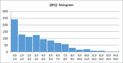
As we can see, after one hour we'll have on average more than 3 customers waiting, if the arrival frequency and service time are as we assumed. So the sporadic nature of arrivals and the service time could cause problems in our barbershop!
We can compare two models quite easily. Copy the results from our model to column C, change the model - for instance, we can add another barber with syQueue(B3,5,B1,2,,1) and run the model once again. After that, we could perfom the t-test or some similar technique to compare the resulting models, but this goes beyond our purpose in this tutorial.
Very clear but less precise way to assess the mean values and dispersion is by creating a chart. If we set our syOutcome's View argument to 6 (syOutcome(B5,B1,6,,1)), Spry will produce a histogram besides the statistics table:
We can also check dispersion throughout the simulation time, by calculating percentiles and displaying a percentiles line chart by setting the View parameter to 2 and 4, respectively (syOutcome(B5,B1,4,,1)):
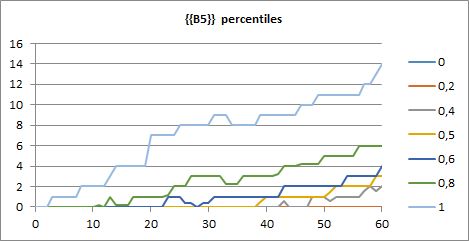
Spry estimates percentiles 0.0, 0.2, 0.4, 0.5, 0.6, 0.8 and 1.0. Besides this, raw values can be displayed by setting the View to 3 (syOutcome(B5,B1,3,,1)):
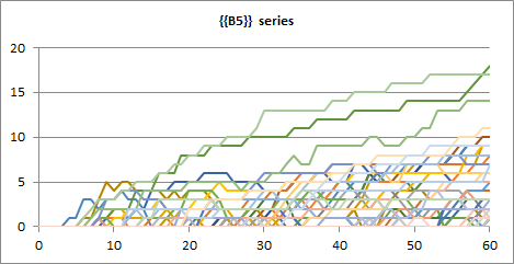
You can equip charts with legeds, titles and also additional data series, as usual in Excel.
Steps in model development
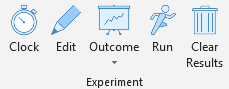
The Experiment group of buttons on the ribbon depicts the steps in model development:
- firstly, we create a clock,
- then we add various elements, creating the model structure,
- we arrange the outcomes (results),
- we run the simulation,
- we compare results with our expectations, if necessary we edit the elements and re-run the simulation.
When we are satisfied with the model, we run the experiments that we are interested in, and finally save results to some safe place.
The validity and functioning of the model is crucial, that's why we build the model in iterations. Usually, we start with the clock with one realization, and add a couple of elements, possibly without stochastics. Then we observe the results with trial runs, proceed with a few additional elements, continuing with trial runs, carefully adding complexity. When we are satisfied with the model, we can run "the real" experiments, with many realizations. During that process, we use syOutcome elements just to check the correctness of the model. These syOutcomes can latter be removed from the model, keepeng just those which directly show the statistics for variables that we are finally interested in.
Tips
Sometimes it's helpful if we formalize and draw the model beforehand. The barbershop case is simple:
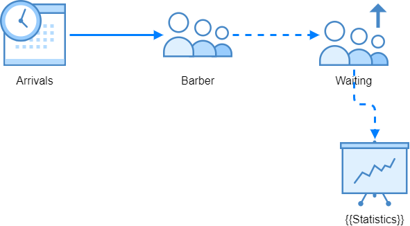
If you'd benefit from this kind of graphic presentations while developing your models, you can download Spry library for draw.io here.
You can download this example from GitHub.