Simulation with Spry
In spreadsheets, modeling is done by expresing model elements and relationships among them by data, formulas and functions in cells. When you make a change in some cell, the recalculation gives immediate response. Spry adds additional functionalities to this concept:
- Technically, it can automatically recalculate the cells in the model for us, according to patterns that we define, or by random number generators, and save the values and statistics of outcome cells after several recalculations for us to analyze.
- Simulation clock is a special cell which introduces time dynamics. It provides current simulation time to other simulation elements throughout the model.
- Simulation time is a foundation for system dynamics and event-driven simulation approaches that are possible by special elements.
Model, simulation time
A model is an abstract representation of a real or artificial system. In spreadsheets we typically create models by a series of formulas in cells. Cells are also used to enter values and quantities that are coming into the model, and model parameters. Parameters are special values that describe the type and strength of relations between variables. We observe resulting cells, typically we try to figure out the right values of parameters so that the model starts to behave according to our desires. Especially important are parameters that we can influence in a real system. The final goal of modeling is to help us to make better decisions.
When you build a model, cells with values, parameters and formulas represent the inner structure of the model. Spry can help you to develop this inner structure, especially by helper functions like random number generators and table function.
To introduce repetitive calculations and dynamic changes, Spry models are always equiped with a clock. The clock defines simulation time - this is the time that our model will live during the simulation. For instance, if we are modeling financial performance of our company for next 4 years, we will set the clock to tick from now to four years in the future. While simulation is running, the simulation time will pass virtually, of course, within our model. To run the simulation, Excel will need a couple or seconds or minutes, depending from the complexity of the model.
During simulation time, Spry is observing the state of the model in regular time intervals. The clock is a special simulation element which is implemented by a syClock() spreadsheet function. Each model can have only one valid syClock(). It defines the length of time intervals, and the start and the end of the simulation time by its parameters TimeInterval, TimeStart and TimeEnd.
Simulation clock and time interval
We can define simulation time in a most simplistic way - if we set just the end, Spry assumes that the time will run from 0 (zero time) to the end time. For example, if we set TimeEnd to 24 and run the simulation, the syClock() will consequtively result in values 0, 1, 2, ... until 24, when the simulation will end. Besides ticking the clock itself, Spry will take note of the model in moments 0, 1, 2, ... and all the consequent moments including the last at 24. In Spry, these moments are called timesteps. Together with timestep 0 this will make 25 model observations.
The length of time interval between timesteps is 1 by default. It is important to note that when we set the TimeStart and TimeEnd parameters to a clock we assume a certain time unit. For instance, if we want to model our company performance on the yearly basis, we set TimeEnd to 4, and simulation time will pass from beginning of the first year (zero time) to the end of year 4. The length of time interval is thus 1 year by default. Spry will log 5 observations.
The time interval can be changed by TimeInterval argument. If we want to observe our simulated company every month, we set the TimeInterval to 1/12 which represents one month. With TimeEnd = 4 we'll get 4 * 12 + 1 = 49 observations.
To conclude, with TimeStart and TimeEnd clock arguments we assume the time unit, while TimeInterval defines the frequency of Spry's observations. This is very important, because when the simulation experiments are done, we have to correctly interpret the results. Besides, some of the Spry elements use the rate of change as input parameters, and these should be given in assumed time units.
Actually, with time functions like TODAY(), NOW() and with Date and Time cell formatting Excel already proposes the general unit of time which is a day. Excel uses the day's serial number (number of days since January 0, 1999). Fractional part represents 24 hour day. We can conveniently use Excel's day time unit by setting TimeStart to the first day and TimeEnd to the last day of the simulation time. Usually, we are not hardcoding dates directly as function arguments, we can prepare both dates in separate cells like:
| A | B | C | |
|---|---|---|---|
| 1 | TimeStart: | 1/1/2022 | |
| 2 | TimeEnd: | 1/31/2022 | |
| 3 | Clock: | =syClock(,B2,B1) |
If we want to be quick with hardcoding, we can also use a neat trick by converting a date string into a number by adding 0 to it:
| A | B | C | |
|---|---|---|---|
| 1 | Clock: | =syClock(,"1/31/2022"+0,"1/1/2022"+0) | |
| 2 |
If we set the number format of the cell with the clock to Date, the syOutcome() element related to that clock will use the date format and display a time series accordingly:
| A | B | C | |
|---|---|---|---|
| 1 | Clock: | 1/1/2022 | |
| 2 | Outcome: | {{B1}} | |
| 3 | 1/1/2022 | ||
| 4 | 1/2/2022 | ||
| 5 | 1/3/2022 |
Shorter time units like minutes, seconds can be also used in this fashion - for instance, if we set =syClock(,"00:00:10"+0,,"00:00:01"+0), we get 10 seconds simulation time by time intervals lasting one second like this:
| A | B | C | |
|---|---|---|---|
| 1 | Clock: | 00:00:00 | |
| 2 | Outcome: | {{B1}} | |
| 3 | 00:00:00 | ||
| 4 | 00:00:01 | ||
| 5 | 00:00:02 |
Because the serial number of ten seconds is 0,000115741, we cannot set only the TimeEnd argument, since Spry would regard TimeInterval as 1 and would "miss" the simulation end time - so we also set the TimeInterval to one second with "00:00:01"+0.
For simlicity reasons, we can always use second as an assumed unit as in =syClock(,10) and not complicate with the format as above. Excel date and time serial numbers and formatting can be useful for demonstrations and publication of results.
Spry supports static models, too. Static models are models without simulation time. To declare static model, set the TimeEnd syClock's argument to be equal to TimeStart. The easiest way is to omit these two arguments in syClock. Model is regarded as static if TimeStart and TimeEnd are equal (e.g. =syClock(,24,24)), however this has no special meaning.
Realizations, experiments
If the simulation model includes stochastic parts, we are dealing with Monte Carlo simulation. This kind of simulation is usually implemented with random number generators. Excel already has inbuild functions like RAND(), RANDBETWEEN() for this purpuse. For convenience, Spry adds syRandomNormal(), syRandomEmpirical(), syRandomDiscrete() and syRandomTriangular() random number generators. Besides this, the syScheduler() element can emit events randomly according to Poisson probability distribution, and syQueue() offers random dispersion of service times. One of the charasteristics of random number genrators in Excel is that they provide a new random number on every spreadsheet recalculation. Formulas that reference those cells change their outcomes accordingly. This is the reason why Monte Carlo simulation models should be calculated several times, and we should check the statistics of outcomes, especially their mean values and dispersion (e.g. average, standard deviation).
Recalculations of all timesteps from start to the end of simulation time are called realization in Spry. We typically use only one realization during the development of the model, because we are checking if the model behaves as it should, and it is easier to spot the error if we have only one realization. When the model is ready for the experiments, the number of realizations should be greater to achieve accurate results. The number of necessary realizations depends from the model itself.
The number of realizations can be set by the syClock() element as the first argument. In this case, syOutcome() elements display the results from all the realizations in a table: timesteps are displayed by rows and realizations by columns (as on the figure below for syOutcome() in B3). syOutcome() elements can also display percentiles (0, 0.2, 0.4, 0.5, 0.6, 0.8 and 1 percentile) by timesteps, and descriptive statistics (average, standard deviation, median, mode, minimum, maximum, kurtosis and skewness) for the last timestep (syOutcome() in F3).
| A | B | C | D | E | F | G | |
|---|---|---|---|---|---|---|---|
| 1 | Clock: | =syClock(3,30) | |||||
| 2 | Triangular: | =syRandomTriangular(1,3,10) | |||||
| 3 | Outcome: | =syOutcome(B2,B1) | =syOutcome(B2,B1,5,,1) | ||||
| 4 | 6.11742 | 6.36685 | 3.67016 | Average | 3.50524 | ||
| 5 | 6.58135 | 3.71770 | 4.52886 | St. dev. | 2.13722 | ||
| 6 | 5.71857 | 8.45179 | 6.16959 | Median | 2.76859 | ||
| 7 | 1.90352 | 7.15414 | 1.98136 | Mode | 0 | ||
| 8 | 3.92415 | 2.00611 | 4.93293 | Minimum | 1.90352 | ||
| 9 | 7.05806 | 8.21732 | 4.21451 | Maximum | 8.45179 | ||
| 10 | 6.01091 | 8.34955 | 2.46689 | Kurtosis | 0 | ||
| 11 | 5.06825 | 2.08872 | 2.44168 | Skewness | 1.54028 | ||
| 12 | 6.29523 | 2.05233 | 2.76859 | ||||
System dynamics
One way of controlling changes in time is the systems dynamics approach. In systems dynamics, three concepts are essential:
- state variables
- rates of change
- feedback loops.
State variables in essence express an absolute quantity that we are observing at certain moment in time (e.g. there are 150 cars in the parking lot, we now have 1200 kg of sugar on stock). Rates of change express changes in states in given time units (e.g. 10 cars per hour are arriving to the parking lot, each day we sell roughly 25 kg of sugar).
In open systems, outputs from the system respond to inputs, however the output has no influence on the inputs. Past action has no effect on the future actions within the system.
In feedback systems, on the other hand, inputs are changed on the basis of outputs. The output in some way is perceived by the system, the decision is made, and action that follows affects the input. In feedback systems, the state variables are influencing rates of change, and rates of change influence state variables in feedback loops. Usually, the changes and influences are not instant but delayed - the material and information takes time to flow from one place to another.
Spry uses continuous time approach to deal with system dynamics numerically, however some concepts of discrete-time systems are added for convenience. Spry elements are following the above ideas. syStock() and syState() represent state variables, they accept rates of change as inputs, which are expressed in time units (some quantity or value per time unit). These two elements accept also discrete changes, that is a change in quantity or value in a certain moment of simulation time. syStock() is meant to be used to model state variables that describe quantities ("material on stock"), syState() is more convenient to express some information in a real system (e.g. the value of some control variable).
Feedback loops can be arranged by syLoop() element. Besides the loop itself, the element also overcomes the Excel's challenge of circular references - if we have a cell's formula that references some other cell which back references the first cell, this leads to an error which is hard to deal with. syLoop() solves this problem in combination with syStock() and syState() elements. syLoop() provides the new rate of change or the new discrete change for syStock() or syState() elements on the basis of the measurements of outputs of these elements in previous timesteps.
Besides states and loops, Spry also provides material and information delays - simplistic linear syMaterialDelay() and syInformationDelay() and non-linear (exponential) types of delays.
Material elements like syStock() and syMaterialDelay() differ from information elements syState() and syInformationDelay() because they preserve the quantities. For instance, material cannot dissapear; if delay time changes then material piles up, however previous information can be "overwritten" by new values.
syStock() element's primary return value is the state, that is the quantity on stock. This is not the only output of this element. Because material is leaving syStock(), the material outflow is also very important. You can get additional outputs from syStock() with syStockOutput() element. Material outflow can then be delayed with syMaterialDelay(), it can be an input to another syStock element and similar.
To illustrate, on the figure below we have Stock A with incoming flow rate of 1 and outflow of 0.5 per hour. syStockOutput() element in cell B3 provides the outflow rate of material that leaves Stock A. This material flow is taken as inflow rate into Stock B. After the simulation run, we can observe changes in all these elements in each timestep provided by syOutcome() elements below row 6. The first syOutcome() in cell A6 points to a clock, so it displays the sequential hours from zero time to 10.
| A | B | C | D | E | F | G | |
|---|---|---|---|---|---|---|---|
| 1 | Clock: | =syClock(1,10) | |||||
| 2 | Stock A: | =syStock(1,0.5,D2,0,0,B1) | =IF(B1=3;2;0) | ||||
| 3 | Stock A output: | =syStockOutput(B2,3) | |||||
| 4 | Stock B: | =syStock(B3,0,0,D4,0,B1) | =IF(B1=7,3,0) | ||||
| 5 | |||||||
| 6 | {{B1}} | {{B2}} | {{D2}} | {{B3}} | {{B4}} | {{D4}} | |
| 7 | 0 | 0 | 0 | 0 | 0 | 0 | |
| 8 | 1 | 0.5 | 0 | 0.5 | 0.5 | 0 | |
| 9 | 2 | 1 | 0 | 0.5 | 1 | 0 | |
| 10 | 3 | 3.5 | 2 | 0.5 | 1.5 | 0 | |
| 11 | 4 | 4 | 0 | 0.5 | 2 | 0 | |
| 12 | 5 | 4.5 | 0 | 0.5 | 2.5 | 0 | |
| 13 | 6 | 5 | 0 | 0.5 | 3 | 0 | |
| 14 | 7 | 5.5 | 0 | 0.5 | 0.5 | 3 | |
| 15 | 8 | 6 | 0 | 0.5 | 1 | 0 | |
| 16 | 9 | 6.5 | 0 | 0.5 | 1.5 | 0 | |
| 17 | 10 | 7 | 0 | 0.5 | 2 | 0 | |
| 18 | |||||||
To make the example more interesting, there is a discrete change of Stock A at time 3 (2 units of material are added) and discrete removal of material from Stock B at time 7 (3 units are removed). This is arranged by simply using the IF() functions in cells D2 and D4 which check if the clock is 3 or 7.
The quantity on Stock A {{B2}} is gradually increasing because of the difference between incoming and outgoing rate (1 vs. 0.5). The outflow from Stock A {{B3}} is constant at 0.5 per hour and it piles up in Stock B {{B4}}.
In the example above we used inflow rates of 1 per hour and 0.5 per hour. Hour was an assumed time unit - as soon as we set the syClock() element as "TimeEnd is at 10 hours", we assumed the unit of time, and in these units we denote TimeStart and TimeEnd of syClock(). This brings consequences also to all systems dynamics elements - all rates of change have to be expressed in the assumed time unit, and don't depend from TimeInterval length.
Discrete Events
Spry supports the concept of discrete events by elements like syScheduler() and syQueue(). An event happens in a certain moment in time. syScheduler() produces events in regular time intervals, with defined frequency as the number of events per time unit. Besides this, it supports random generation of events (Poisson process).
In their way through the system, events can be delayed. This is one of the purposes of syQueue() element. Actually, syQueue() is more than that. Internally, it consists of servers and one waiting line. Servers work in parallel and are engaged by incoming events, for the specifed ServiceTime. With this, the internal structure of syQueue() element follows the ideas of queuing theory. ServiceTime can be stochastic and defined according to Erlang probability distribution.
The return value of syScheduler() and syQueue() is the number of events emitted in the last time interval. If you reference that value by some other formula or Spry element, you can create a path between event generators and servers. A gateway, i.e. a split of the "pipeline" of events into two or more paths can be easily created by IF() functions, as seen from the following figure.
| A | B | C | D | E | F | G | H | |
|---|---|---|---|---|---|---|---|---|
| 1 | Clock: | =syClock(1,240) | {{B3}} | {{B5}} | {{B6}} | {{B7}} | {{B8}} | |
| 2 | Scheduler: | =syScheduler(5,3,B1)) | 0 | 0 | 0 | 0 | 0 | |
| 3 | Queue A: | =syQueue(B2,2,B1,6,,1) | 4 | 0 | 4 | 0 | 4 | |
| 4 | Split: | =RAND() | 6 | 6 | 0 | 6 | 0 | |
| 5 | - to Q_B1: | =IF(B4<=0.3,B3,0) | 6 | 0 | 6 | 0 | 6 | |
| 6 | - to Q_B2: | =IF(B4>0.3,B3,0) | 5 | 0 | 5 | 0 | 5 | |
| 7 | Queue B1: | =syQueue(B5,10,B1,,,1) | 3 | 0 | 3 | 0 | 2 | |
| 8 | Queue B2: | =syQueue(B6,2,B1,,,1) | 6 | 0 | 6 | 0 | 7 | |
| 9 | 6 | 0 | 6 | 0 | 13 | |||
| 10 | 6 | 6 | 0 | 6 | 0 | |||
RAND() function in cell B4 "decides" about the path that the events in particular timestep will follow, which is done by two IF() functions in B5 and B6. If RAND() gives a number less or equal to 0.3 threshold value, the events are routed to Queue B1, otherwise they continue their way to Queue B2. syOutcome() elements {{B5}} and {{B6}} show which way the events from Queue A were following at particular timestep. In this way, we implemented the fact that 30 % of all events on average should go to Queue B1.
The "join" gateway is quite easy, you just add two paths together, like =B7+B8 to join the events coming from Queue B1 and Queue B2.
In systems dynamics elements like syStock() and syState() we have discrete changes that represent a specific quantity or value that is added or removed from the state. Events coming from syScheduler() and syQueue() can be used to moderate these discrete changes. Some absolute quantity (e.g. number of ordered items) can be multiplied by the number of events in particular time interval (e.g. one order) and feed into the syStock() and syState() elements as DiscreteInflow, DiscreteOutflow, and DiscreteChange.
We already mentioned the assumed time units and their importance for systems dynamics. With discrete evetns, we have to be careful with the interpretation. The results of discrete events elements in general represent the number of emitted events in the last time interval. syScheduler's Rate argument should be used as a rate of events per assumed unit of time, similar to the rates of change in systems dynamics elements. In this fashion, the rate 12 means 12 evens per unit of time, and 3/12 means three events per 12 units of time.
Here follows somewhat sophisticated example, where the simulation time is from 0 to 3 hours, and the time interval is set to one minute, that is 1/60 of an hour (in syClock()):
| A | B | C | |
|---|---|---|---|
| 1 | =syClock(,3,,(1/60)) | ||
| 2 | =syScheduler(7/(10/60),1,A1) | ||
| 3 | {{A1}} | {{A2}} | |
| 4 | 0 | 0 | |
| 5 | 0.0166667 | 0 | |
| 6 | 0.0333333 | 1 | |
| 7 | 0.05 | 1 | |
| 8 | 0.0666667 | 0 | |
| 9 | 0.0833333 | 1 | |
| 10 | 0.1 | 1 | |
| 11 | 0.1166667 | 0 | |
| 12 | 0.1333333 | 1 | |
| 13 | 0.15 | 1 | |
| 14 | 0.1666667 | 1 | |
| 15 | 0.1833333 | 0 | |
In syScheduler(), we declared 7 events per every 10 minutes (7 per 10/60). Spry generates events is such a way that they are spread evenly as much as possible over the given time interval within the rate. As we see above , there were exactly 7 events emitted until 0.1666667, which represents the first 10 minutes of an hour (10 / 60 = 0.1666667)
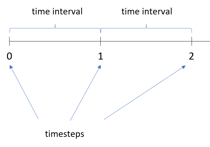
TimeSteps, TimeIntervals
In dynamic simulation models we have to deal with time intervals and timesteps. Time interval is the duration of simulated time between two timesteps. At every timestep, Spry checks the state of all the variables in the model and makes recalculations. The image below shows the first three timesteps denoted by 0, 1 and 2 serial numbers that are by one time interval "apart" from each other.
All elements, including syOutcome() present their values at a certain timestep. Each value is the evidence of happenings in the model within the last time interval. This is true also for resulting rates of changes. For instance, the outflow rate from syStock() which we can get by syStockOutput(some_syStock, 3) is the rate of change per unit of time that was measured in the last time interval.
If an event is generated at exactly the timestep, it counts as a result of the previous time interval. From the picture below, we can see that events b, c and d were generated after timestep 3 until (and including) timestep 4. Spry accounts this as three events reported at timestep 4. The event a that was emitted exactly at timestep 3 counts for the previous time interval and is reported at timestep 3.
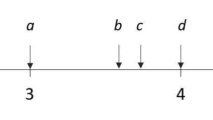
If you want to get very exact results (for instance, if you'd like to know how huch apart are events b, c and d) then you could make the time interval shorter, however the number of timesteps can become enormously high and Spry would need a lot of time to process all the details.
Optimization
There are many reasons for using simulations. We can study the functionings of the real system, and perform simulations to demonstrate our understanding of the system. Frequently, we use simulation studies to compare two models, for instance as-is model and to-be model, when we are proposing some changes to stakeholders. Typically, we observe one or more outcomes of the model (the outcome values at the end of simulation time) and compare their mean values. This comparisson can be graphical (e.g. by comparing histograms) or exact with estimating the necessary statistics, like t-tests and other comparissons.
Often, we are searching for some optimal value that we would like to use in business practice. Excel offers a couple of optimization tools, for instance What-If Analysis and Solver add-in.
Spry can be used in combination with Solver add-in. In essence, Solver iteratively changes variable cells according to constraints, observes the objective cell and searches for the optimal combination of variable cells values.
Simulation model in Spry can be used to recalculate the outcome that is observed by Solver. For that purpose, we have to "expose" variable cells in Spry. Variable cells should represent some parameters within our simulation model that Solver will change repeatedly. After each change of these cells by the Solver, Spry will automatically run the simulation, all the realizations. You can use the syExposeVariableCells() function to expose the variable cells in this fashion.
The objective cell should be set in Solver to one of the results of the simulation model. For this purpose, it's best to use syStatistic() function which returns one of the statistics for a chosen outcome cell. Available statistics are average, standard deviation, median, mode, minimum, maximum, kurtosis, and skewness.
Another way to try out various combinations is to use Scenario Manager, however changing the scenario doesn't automatically run the simulation, so there is no need to expose variable cells with syExposeVariableCells() in this case.