Getting started with Spry Simulations

Spry brings to MS Excel additional spreadsheet functions that represent event generators, queues, state variables, delays, loops and other simulation elements that you can connect together while designing the model in spreadsheet.

During simulation run, Spry mimicks the passage of time by recalculating the model several times, for each consequtive time period. Data collection and statistics for specific cells in the model that interest you is also arranged as a spreadsheet function. Besides this, simulation models usually include stochastic variables, so to get reilable results Spry can repeat the whole model several times.

Simple call center example

Suppose we have a call center where a new call from customers happens every 2 minutes. We have two colleagues in the center and they need 5 minutes on average to complete each call. How many customers can they respond to in 2 hours?

Our task is to generate calls and process them, together with collecting the statistics. This can be done by syScheduler(), syQueue() and syQueueOutput() functions like in the animation below.

Firstly, we need a simulation clock, so we use syClock() function and set it to simulate two hours (which is 120 minutes) of call center activities:

B1: =syClock(,120)

Calls are being generated by the scheduler. The rate is one call per two minutes (1/2) and calls are generated in regular intervals, where the first call happens right at the beginning of simulation:

B3: =syScheduler(1/2,2,B1)

Calls are then "fed" into the queue which consists of a waiting line and servers - we have 2 colleagues (two "servers"), and because the service time should be sporadic with average service time of 5 minutes, we use exponential dispersion:

B4: =syQueue(B3,5,B1.2,,1)

To count for the served customers, we use syQueueOutput() which points to our queue and where we choose (with the second parameter) cumulative number of events coming from the queue:

B5: =syQueueOutput(B4,1)

While Spry runs the simulation, it recalculates these functions several times during the simulation time - once per each simulated minute. At the end of simulated time, the functions keep their final values, like total number of customers. However, if we'd like to observe our call center during the simulated time, we use the syOutcome() function:

A7: =syOutcome(B5,B1,3)

The View parameter of 3 means that we will get a timetable of all the values of cell B5 (cumulative number of served customers) together with a chart with this dataseries.

Because the service time is sporadic, we deal with Monte Carlo approach, that's why we need to repeat the simulation. This is easy in Spry - we just set the number of repetitions in the clock:

B1: =syClock(5,120)

If we run the simulation again, the chart displays all five data series. At the end we get the statistics (average, std. deviation etc.) of customers served in two hours by:

J7: =syOutcome(B5,B1,5,,1)

As View parameter we have 5 (Statistics). Last parameter TableDescriptions of 1 annotates the statistics table with names of parameters, so we have no troubles with the interpretation.

Of course, we can change the parameters (for instance the number of colleagues in call center) to try various solutions.

Chaotic system example

Let's simulate a simple chaotic system where its state in the next time period is defined as

state_t+1 = parameter * state_t * (state_t - 1)

The rate of change is thus

parameter * state_t - parameter * state_t² - state

Because the rate of change depends from current state and influences the future state, we have a feedback loop:

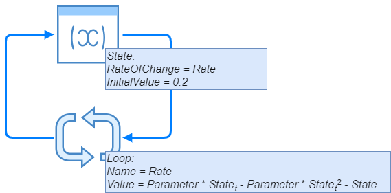
By using Spry, we can implement this chaotic system by syState() and syLoop() functions and initial state of, let's say 0.2 like this:

Apart from syState() and syLoop() functions, we use syClock() to define the time dimension (simulation time lasts 50 time units), and syOutcome() which displays the resulting states and a chart. So, we have these formulas:

B1: =syClock(,50)

B2: 2

B3: =syState("Rate",0,0.2,B1)

B4: =syLoop("Rate",B2*B3-B2*B3^2-B3)

B6: =syOutcome(B3,B1,3)

By changing parameter values and running the simulation we can see how the system reacts to the parameter change. You can download this example from GitHub.

Installation

Setup is simple. Please download the installer and follow the instructions to obtain trial or permanent licence.

Further steps

After installation, you can immediately start building models as above. To make this easier, you can follow the discrete-event simulation tutorial which demonstrates the Spry approach to simulations with a simple model. System dynamics simulation is presented by Bass adoption model example tutorial that follows. A mixed approach with optimization is illustrated by an example of inventory management.

For further reference, please have a look at additional information about Spry together with functions' reference, while deeper exploration of what can be done with Spry is given on Simualation with Spry page.